Before you start…
Make sure you are still in your project that you created for doing exercises and then make a new R script. Save it as soon as you make it and give it a good name like exercise_1_day_4.R or franz.R and you’ll be ready to go!
Day-dreams
All these flightless birds have been making us think…if we were a bird who could fly, where would we go? Would we follow other birds or would we make your own path? Where is home when you can fly?
One of these days we’ll learn our lesson about asking questions, but for now we have endless curiosity and a need to know.
The pillars of spatial analysis in R
- sf for spatial functions
- tigris for geographic boundaries
- ggplot2 or leaflet for map making
- tidycensus for Census data
In this exercise we will analyze a bird flight path. Our steps will be as follows:
- Make two point geometries representing trees.
- Make a line geometry.
- Make a polygon geometry.
- Read in U.S. state boundaries.
- Make a map with the state boundaries and the flight path.

Say you want to measure how far a bird must fly from their nest in St. Paul, MN down to the center of Smoky Mountain National Park in Tennessee.
Let’s set up 2 points, and then measure how far apart they are. Next we will develop a polygon that is a straight path between these two nesting locations and join with the states to develop a final list of states that the birds will fly through and make some maps. We’ll leave it to you to develop strict conservation laws to protect the trees along this important flight path.
It begins.
A tree stands in the center of St. Paul
First we set up the simplest point data, a single point with a latitude and longitude. The st_as_sf function will convert the dataframe to an sf (simple feature) object and assign it a coordinate reference system (CRS).
# Only need to run this once
install.packages("sf")
library(sf)
library(tidyverse)
# Latitude is like a ladder, up and down, north to south
lat_y <- 44.928397
long_x <- -93.173445
nest_mn <- data.frame(nest = "MN",
longitude = long_x,
latitude = lat_y)
nest_mn <- st_as_sf(nest_mn,
coords = c("longitude", "latitude"), # Longitude column goes first!
crs = 4326, # Provide the coordinate reference system
remove = FALSE)A tree stands in the center of Smoky Mountain National Park
Now we make another point in Tennessee. Remember points are singular geometries and have no area. Sometimes, if you are attempting to intersect points with polygons, you may have to draw a buffer around them.
lat_y <- 35.581196
long_x <- -83.860947
nest_smnp <- data.frame(nest = "SMNP",
longitude = long_x,
latitude = lat_y)
nest_smnp <- st_as_sf(nest_smnp,
coords = c("longitude", "latitude"),
crs = 4326,
remove = FALSE) # Keeps the original coordinate columnsHow far apart are these two nests? We need to convert the coordinate reference systems to make sure that the two locations are comparable and our final answer is in meters. You can change coordinate reference systems by using the function st_transform.
Next we use the st_distance. Since we are using a coordinate reference system with units in meters, our distance units will be meters as well. So, we can convert to kilometers by dividing by 1,000.
# Transform the projections
nest_mn <- st_transform(nest_mn, crs = "ESRI:102003")
nest_smnp <- st_transform(nest_smnp, crs = "ESRI:102003")
# Calculate the distance between them in meters
tree_distance_m <- st_distance(nest_mn, nest_smnp)
# Kilometers
tree_distance_km <- tree_distance_m / 1000
Click here to view the full PDF
We will make a dataframe with our two nest points by binding the two points together as rows of a table using bind_rows.
Then we’ll say that the birds will fly in roughly a straight line. So we can cast these two points into a line by first joining them using st_union and then casting them to a “linestring” (this is a line geometry) using the st_cast function.
tree_points <- bind_rows(nest_mn, nest_smnp)
tree_route <- tree_points %>%
summarize(geometry = st_union(geometry)) %>%
st_cast("LINESTRING") %>%
mutate(route = "Minnesota to Smoky Mountain National Park")
plot(tree_route)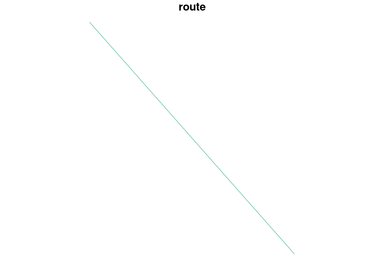
We can be fairly sure the birds won’t fly in an exactly straight line from Minnesota to Tennessee. So, let’s put a buffer around this line. This will make it a polygon object. Let’s assume the birds will fly within 20,000 meters around our entire line.
Let’s double check that our route’s projection has units in meters or metres, and then add a 20,000 meter buffer. It will be glorious.
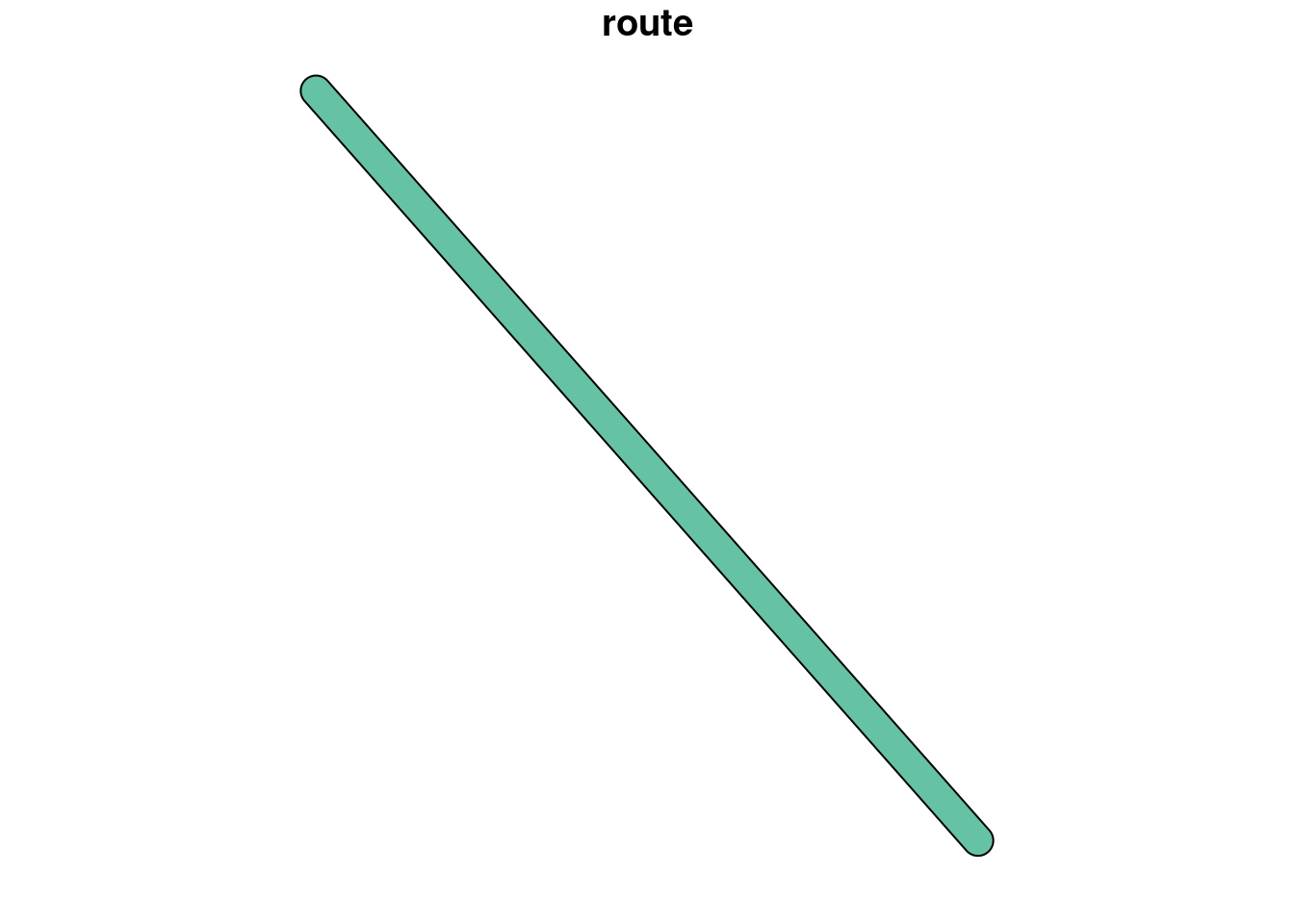
Looking at that shape in our plots window is a bit underwhelming. Sorry plot function, but I want to see what states the flight path goes through, and I’d eventually like a map to use as a reference. So, let’s get started.
First, we are going to pull in our tigris package and get polygons of the state boundaries.

Now let’s see which states intersect with our polygon bird path. We bring back some sf magic for this. But remember, the CRS must be the same!! SO, we will need to do some transformation. This time we use st_crs to transform one geometry to the CRS of the other one. Then we can use st_filter to filter one geometry to the extent of the other.
States flown over
Check the CRS for each object and transform them if necessary to make them match. Then use st_filter to find the states that intersect with the bird path.
st_crs(all_states) st_crs(tree_route) all_states <- st_xxxx(all_states, crs = _________) bird_route_states <- st_filter(_______ , _________)
st_crs(all_states) st_crs(tree_route) all_states <- st_transform(all_states, crs = st_crs(tree_route)) bird_route_states <- st_filter(all_states, tree_route)
Now we have two types of polygons, a set of states that intersect with our bird path and the bird flight path itself. We will make a map of these two shapes in two ways. First with leaflet then with ggplot2.
Leaflet prefers coordinates to be in Lat/Long. No problem. We can use st_transfrorm on the fly in our leaflet pipeline.
library(leaflet)
leaflet() %>%
addTiles() %>%
addPolygons(data = st_transform(bird_route_states, crs = 4326)) %>%
addPolygons(data = st_transform(tree_route, crs = 4326), weight = 5, color = 'darkorange')![]()
Now, let’make a ggplot map. Time to flex those ggplot muscles from last session! We’re going to add a few new geoms to our toolbox: geom_sf and geom_sf_text.
Maps with ggplot
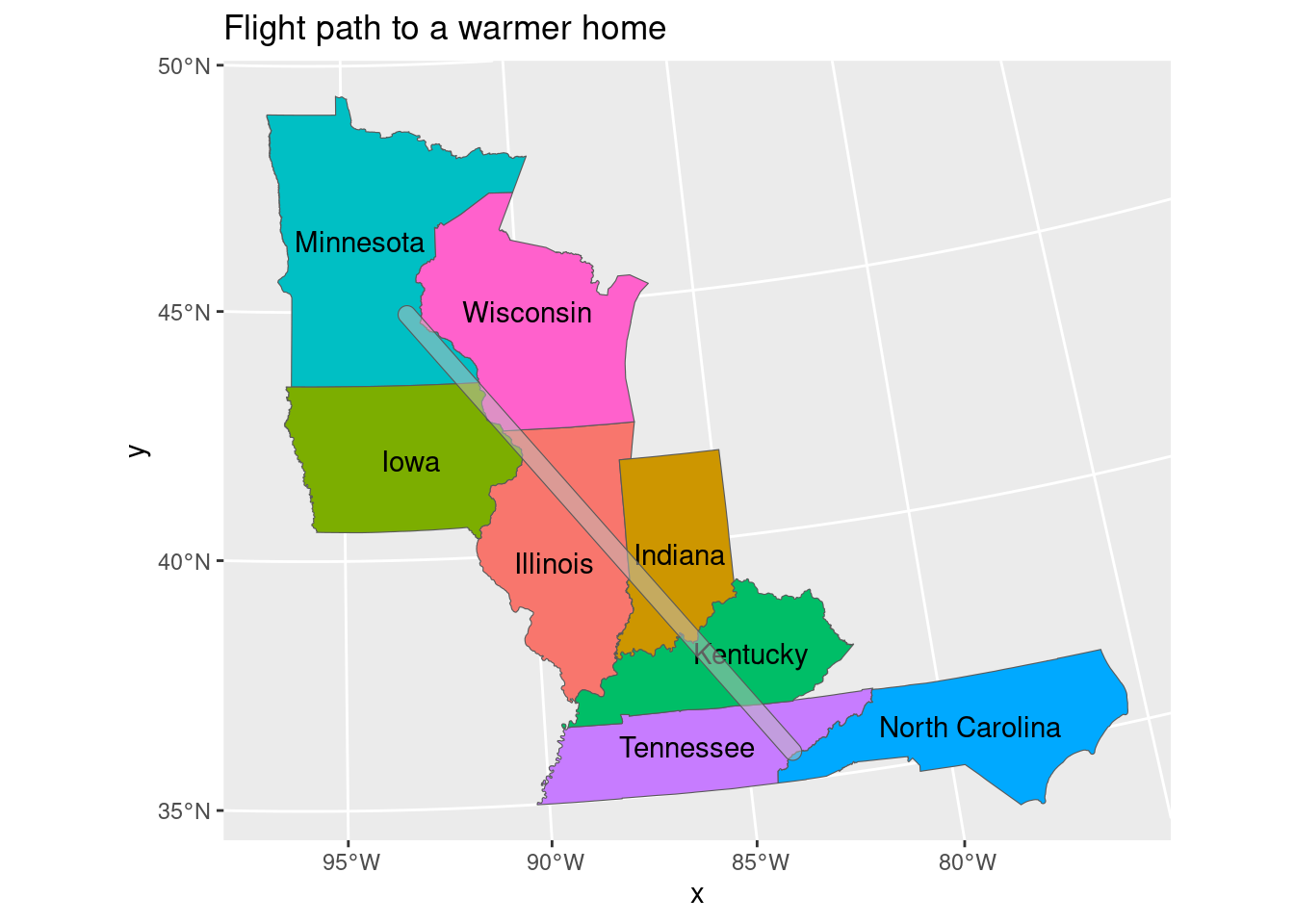
Make a map of the flight route with the state boundaries underneath. Use geom_sf to plot the shapes and use geom_sf_text to add labels to the states.
ggplot(bird_route_states) + geom_sf(aes(fill = ______ )) + geom_sf_text(aes(label = ______ )) + geom_sf(data = ________ )
ggplot(bird_route_states) + geom_sf(aes(fill = NAME), show.legend = TRUE) + geom_sf_text(aes(label = NAME)) + geom_sf(data = tree_route, alpha = 0.5) + labs(title = "Flight path to a warmer home")
Don’t forget the important work left to do on conservation efforts: What states would need to be informed about the flight pattern and nesting behavior? What data could you give them to make their job easier? What might you do to expand on the work that we have already done to better answer any questions from legislators?
