Before you start…
Make sure you are still in your project that you created for doing exercises and then make a new R script. Save it as soon as you make it and give it a good name like exercise_2_day_4.R or katya.R and you’ll be ready to go!
Building on our previous work…
Now that we know where the birds go, we need to make sure that they have a safe and healthy home to go to!
Let’s check out the health of the forest by county in the state of Minnesota. We will need to know the locations of the counties in Minnesota, and we will also need some forest health data.
The Minnesota Geospatial Commons is an excellent source of geospatial data in Minnesota and is very searchable.
If you search forest health you will find some forest health datasets of large scale tree canopy damage prepared for several years. We will use the most recent, 2022. Let’s read in a shapefile using the sf package. You will note that the shapefile is [zipped](https://en.wikipedia.org/wiki/ZIP_(file_format). So we first create two temporary folders to begin the process of grabbing this file, unzipping it, and then reading it in as a simple feature (sf) object. The temp and temp2 folders, and the shapefile, is saved in a local temporary folder.
If you want to save the shapefile on your computer for the longterm, you can use the st_write function.
library(tidyverse)
library(sf)

# Create temp files
temp <- tempfile()
temp2 <- tempfile()

# ZIP file URL
url <- "https://resources.gisdata.mn.gov/pub/gdrs/data/pub/us_mn_state_dnr/env_forest_health_survey_2022/shp_env_forest_health_survey_2022.zip"

# Download the zip file and save to temp
download.file(url, temp)

# Unzip the contents of the temp and save unzipped content in temp2
unzip(zipfile = temp, exdir = temp2)

# Read the shapefile
forest_damage <- st_read(temp2)
## Reading layer `forest_health_survey_2022' from data source
## `/tmp/RtmpGIdYlq/file6016cd70e27' using driver `ESRI Shapefile'
## Simple feature collection with 2825 features and 10 fields
## Geometry type: POLYGON
## Dimension: XY
## Bounding box: xmin: 194139.8 ymin: 4998795 xmax: 748411.6 ymax: 5467028
## Projected CRS: NAD83 / UTM zone 15NWe can look at the data in two ways:
- View the attributes by clicking
forest_damagein the Environment pane. Look at the geometry column. That is where the spatial information is stored. Each row in the dataset is a different polygon shape, but all belong to the same dataset or shapefile. - Next, we can plot the data in base R to make sure it has the appropriate geographic information and at least looks like a map. This is a good first check to see if you’ve successfully pulled in the proper shapefile.
When we look at this, we see that there are many polygons, and if we look at the data (by running glimpse(forest_damage), or clicking on forest_damage in the environment) we see that there are severity ratings for each polygon in the column PERCENT_AF.
For our first analysis let’s sum the area in each county that has damage to tree canopy. Then, we can bring in another county dataset to look at the places in MN with the most tree canopy damage and see if our bird’s flight path has been affected. For step one, let’s use tigris and pull in the county shapefile for Minnesota.
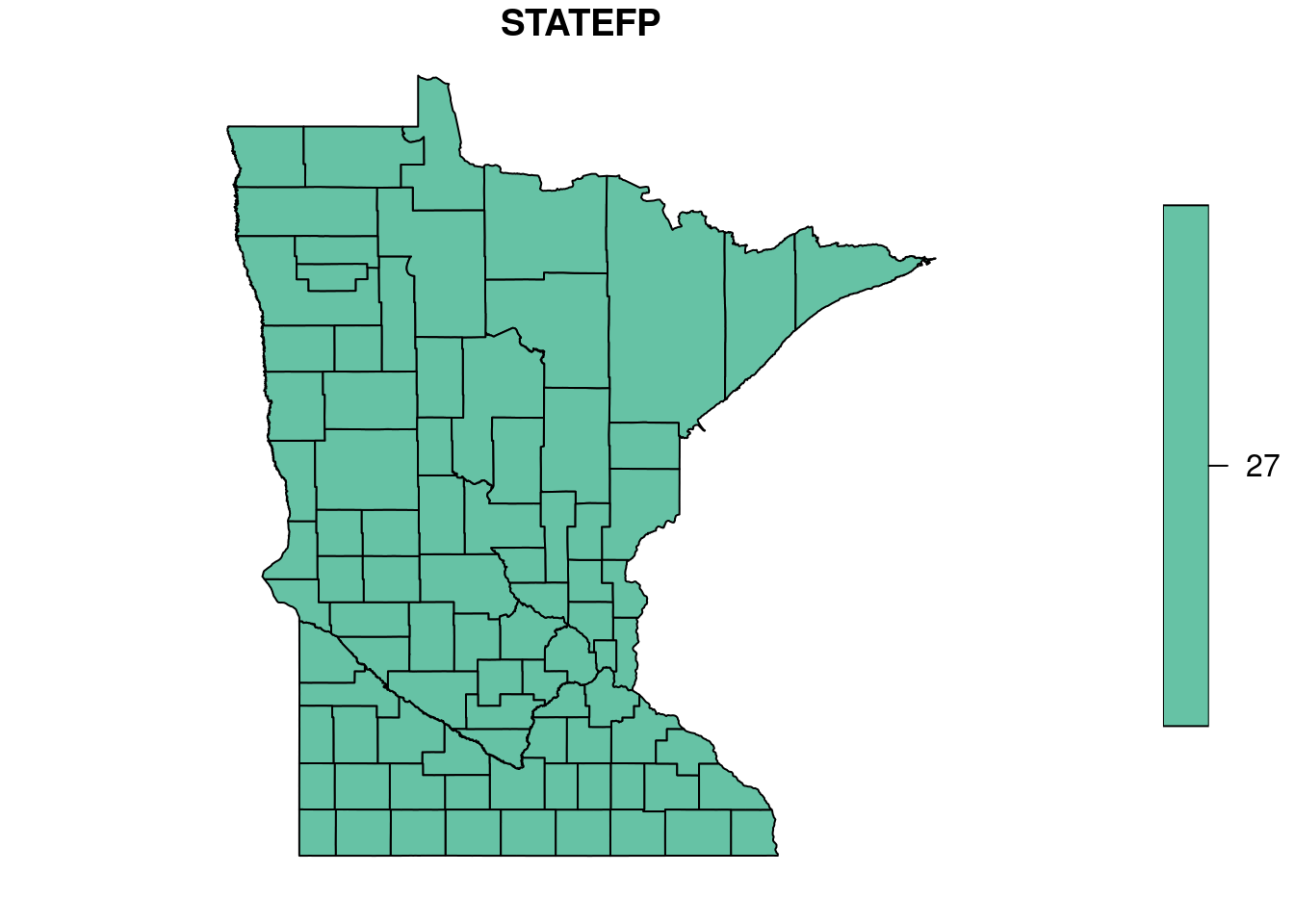
And of course we want to check to see if our CRS match, because we want to join these two geospatial datasets.
The forest damage dataset has a coordinate reference system in UTMs (Universal Transverse Mercator), and remember that those have units of meters, which are very nice for working with area measurements. So, let’s convert the county dataset into UTMs as well. Zone 15 is Minnesota’s primary UTM zone, and the ID for UTM Zone 15 is 26915.
Now, we can run a spatial intersect on the two geospatial datasets. The st_intersection function returns the polygons where the two geometries intersect. (Here’s a short description with images.) All of the polygons in the forest_damage dataset will be split into their respective Minnesota county. So, some of the forest damage polygons may be split across several counties. But no worries, R has us covered!
## Warning: attribute variables are assumed to be spatially constant throughout
## all geometries
Take a look. The forest polygons that spanned across county borders have been split into two polygons.
An original forest damage polygon from row 2,011 in the forest_damage data.
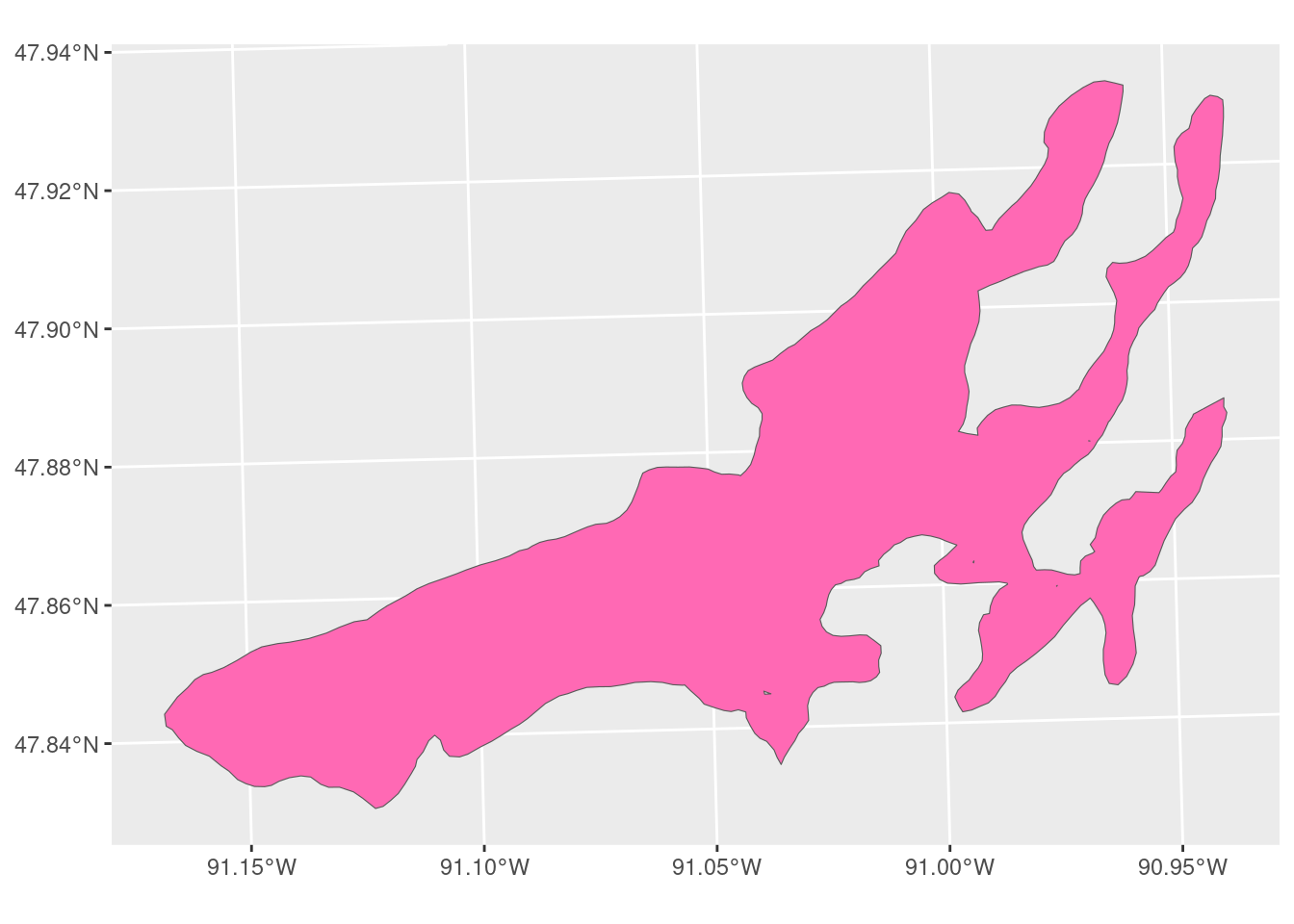
The shape was split into two polygons along the county border when intersected with the counties data.
ggplot() +
  geom_sf(data = forest_damage_counties["2011", 1], fill = "green") +
  geom_sf(data = forest_damage_counties["2011.1", 1], fill = "darkgreen")
## Error in `calc_limits_bbox()`:
## ! Scale limits cannot be mapped onto spatial coordinates in
## `coord_sf()`.
## ℹ Consider setting `lims_method = "geometry_bbox"` or `default_crs = NULL`.st_area
Next, we can calculate the area for each of the new split up forest_damage polygons.
Since we no longer need each individual polygon geometry, we can set the geometry of the dataset to NULL. This can help save some memory for R when working with large datasets.
Check the dataframe to see if the
geometrycolumn vanished. I hope so!
Now, we want to sum the damaged tree area within each county. This will be a throwback to our group_by and summarize work. We want our new summarized dataframe to have the following information: the total area in the polygon and the name of the county.
Sum up the damaged areas
We are going to sum the damaged areas within each county, returning the following information: the total area in the polygon and the name of the County. Call the summarized data forest_damage_total.
forest_damage_total <- forest_damage_counties %>%
  group_by(______) %>%
  summarise(total_damaged_area = __________)
forest_damage_total <- forest_damage_counties %>%
  group_by(NAME) %>%
  summarise(total_damaged_area = sum(damage_area, na.rm = TRUE))
Join tables
Now we need to join the summed forest damage data to the county spatial data so that we have the information we need to present the data as a map. We use left_join below to add the forest damage totals to the county polygons. The rows are joined based on where the county names match in both tables in the NAME columns. We’ll cover joins in great detail next session - so consider this a preview teaser.
Should the missing values for damaged area be zero?
Now, we replace all missing values with zeroes. You always want to think a bit before replacing NULLs with zeroes. In this case, we have some information to justify that the missing values are where there was no forest canopy damage and so the forest canopy damage area would be zero (based on the reports used in this dataset).
Sometimes a NULL means there is no information, which means that you don’t know what the value is and you do not have adequate information for replacements.
## Error in eval(expr, envir, enclos): object 'county_totalse' not foundOh, right! Our area column has units attached and is not a simple number. We could convert the column to
as.numericor we can replace the NA values with a value that has units, such as0 m^2. Let’s do that with theunitspackage.
library(units)

county_totals <- county_totals %>%
                 mutate(total_damaged_area = replace_na(total_damaged_area, as_units(0, "m^2")))
Okay that was fun, but now let’s drop the units entirely. They don’t really play that nice with ggplot and leaflet. They’re always like, just show me the raw numbers!
# Drop the units
county_totals <- county_totals %>%
  mutate(total_damaged_area = as.numeric(total_damaged_area))
Finally we get to make a map. Remember, data prep is more than half the battle!
Map it out
Make a map using ggplot and geom_sf. Remember to add good plot elements like titles and colors. Fun colors are very important.
What should you add to make this a more complete plot?
ggplot(data = ________, aes(fill = total_damaged_area)) +
  geom_sf()
ggplot(data = county_totals, aes(fill = total_damaged_area)) +
  geom_sf()+
  labs(title = "Total forest canopy area damage",
       subtitle = "Minnesota counties",
       x = "Longitude",
       y = "Latitude",
       caption = "Source: 2022 MN DNR Forest Health Survey") +
  scale_fill_viridis_c(name = "Total Damaged Area") +
  theme_minimal()
Our bird originated in St. Paul, MN and it looks like there wasn’t a lot of damaged forest canopy in Ramsey county. So I’m going to assume our bird is whistling away in a healthy little tree.
Happy spatial analysis friends!