Getting started
- Create a new R script.
- Save it and give it a good name like
5-2_exercise.Rortemp_analysis.R. - You’re ready to go!
The question
The research crew wants to determine if there is a relationship between isotope levels in the penguins_raw data and temperature. We have temperature data for each of the islands uploaded to the webpage.
Let’s get all of this temperature data into R first, and then we can combine it with our penguins_raw data.
Data exploration
Let’s do a quick overview of our temperature data. As you are exploring the data, look for what is different between the 3 data frames?
What are some things we could do to make the data more tidy?
Clean-up time
Step 1
Take a closer look at the torg data. Why does it have so many more rows? Try arranging the data by the date column, what do you notice?
## # A tibble: 2,192 × 2
##    date       temperature_c
##    <date>             <dbl>
##  1 2007-01-01           1.5
##  2 2007-01-01           1.5
##  3 2007-01-02           1.3
##  4 2007-01-02           1.3
##  5 2007-01-03           4.1
##  6 2007-01-03           4.1
##  7 2007-01-04          -0.3
##  8 2007-01-04          -0.3
##  9 2007-01-05           2.3
## 10 2007-01-05           2.3
## # ℹ 2,182 more rows
Icky…It looks like there are duplicate rows in the data. That seems to happen a lot. Since the temp value always appears to be the same for the duplicate row, I think it is safe to say the duplicate should be removed.
If you are 100% sure your data should not have duplicate rows in it, you can use the function distinct( ) to keep only one row from each of the groups of duplicates. In the end, every row will be a distinct and unique row compared to ALL others in the table.
How many rows does torg have now?
Step 2
The island names are in the file name, but are not in the data itself. That’s not ideal when you’re looking to join data together or perhaps want to label points on a chart with the island name.
Let’s add the island names to use for joining later. Remember that R is picky about name matching, so it’s important to make sure the names are exactly correct, including CAPs.
The island names are Biscoe, Dream, and Torgersen. Copy/Paste is your friend here. Use mutate( ) to add a new column called island to each of the data sets.
Which island?
Use mutate( ) to add a new column called island to each of the data sets.
biscoe <- biscoe %>%
          mutate(island = ______ )

dream <- dream %>%

#.....
biscoe <- biscoe %>%
          mutate(island = "Biscoe")

dream <- dream %>%
         mutate(island = "Dream")

torg <- torg %>%
        mutate(island = "Torgersen")
When exploring the data, did you notice anything about the dates? They are all in different formats! Luckily we have lubridate to come to the rescue. Let’s convert those dates so they are all in the same format. Remember to choose your date function from the table below.
| Format | Function to use |
|---|---|
| Month-Day-Year ~ “05-18-2023” or “05/18/2023” | mdy(date) |
| Day-Month-Year ~ “18-05-2023” or “18/05/2023” | dmy() |
| Year-Month-Day ~ “2023-05-18” or “2023/05/18” | ymd() |
Make it a Date
Use mutate( ) to convert the date column to a Date object in each of the data sets.
biscoe <- biscoe %>%
          mutate(date = mdy(date))

dream <- dream %>%
         mutate(date = ________ )

#.....
biscoe <- biscoe %>%
          mutate(date = mdy(date))

dream <- dream %>%
         mutate(date = dmy(date))

torg <- torg %>%
        mutate(date = ymd(date))
Binding them all together
To join the temperature data to our penguin data easily, we want to combine all 3 data frames into one data frame. Keeping in mind tidy data, what is the best way to do this?
Run a few tests on the new table to ensure all the island data survived the bind_rows journey.
More data exploartion
We have our temperature data in a happy place, but what about the penguin data? Let’s get the data and determine which columns we can use to combine with our temperature data.
## Rows: 344
## Columns: 17
## $ studyName             <chr> "PAL0708", "PAL0708", "PAL0708", "PAL0708", "PAL…
## $ `Sample Number`       <dbl> 1, 2, 3, 4, 5, 6, 7, 8, 9, 10, 11, 12, 13, 14, 1…
## $ Species               <chr> "Adelie Penguin (Pygoscelis adeliae)", "Adelie P…
## $ Region                <chr> "Anvers", "Anvers", "Anvers", "Anvers", "Anvers"…
## $ Island                <chr> "Torgersen", "Torgersen", "Torgersen", "Torgerse…
## $ Stage                 <chr> "Adult, 1 Egg Stage", "Adult, 1 Egg Stage", "Adu…
## $ `Individual ID`       <chr> "N1A1", "N1A2", "N2A1", "N2A2", "N3A1", "N3A2", …
## $ `Clutch Completion`   <chr> "Yes", "Yes", "Yes", "Yes", "Yes", "Yes", "No", …
## $ `Date Egg`            <date> 2007-11-11, 2007-11-11, 2007-11-16, 2007-11-16,…
## $ `Culmen Length (mm)`  <dbl> 39.1, 39.5, 40.3, NA, 36.7, 39.3, 38.9, 39.2, 34…
## $ `Culmen Depth (mm)`   <dbl> 18.7, 17.4, 18.0, NA, 19.3, 20.6, 17.8, 19.6, 18…
## $ `Flipper Length (mm)` <dbl> 181, 186, 195, NA, 193, 190, 181, 195, 193, 190,…
## $ `Body Mass (g)`       <dbl> 3750, 3800, 3250, NA, 3450, 3650, 3625, 4675, 34…
## $ Sex                   <chr> "MALE", "FEMALE", "FEMALE", NA, "FEMALE", "MALE"…
## $ `Delta 15 N (o/oo)`   <dbl> NA, 8.94956, 8.36821, NA, 8.76651, 8.66496, 9.18…
## $ `Delta 13 C (o/oo)`   <dbl> NA, -24.69454, -25.33302, NA, -25.32426, -25.298…
## $ Comments              <chr> "Not enough blood for isotopes.", NA, NA, "Adult…
Both data frames have an island column and a date column, but with different names. What operation do we want to use? Which join type is most appropriate here? Remember that when combining data frames, column names are important and are case-sensitive. We want the resulting data frame to have the same number of rows as the penguins_raw data frame.
Table join
Use a ****_join( ) function to combine the columns of the two data sets so the result has the same number of rows as penguins_raw.
penguin_temps <- left_join(penguins_raw, temps,
                           by = c("Island" = "_______" ,
                                  "Date Egg" =  "______" ))

# inner_join() would also work in this case
penguin_temps <- left_join(penguins_raw, temps,
                           by = c("Island" = "island",
                                  "Date Egg" = "date"))
The relationship between temp and isotopes
With all of the data in one data frame, we can now plot isotope levels versus temperatures. But first, we need to clean up those long tricky column names. How do we do that?
##  [1] "studyName"           "Sample Number"       "Species"
##  [4] "Region"              "Island"              "Stage"
##  [7] "Individual ID"       "Clutch Completion"   "Date Egg"
## [10] "Culmen Length (mm)"  "Culmen Depth (mm)"   "Flipper Length (mm)"
## [13] "Body Mass (g)"       "Sex"                 "Delta 15 N (o/oo)"
## [16] "Delta 13 C (o/oo)"   "Comments"            "temperature_c"
#install.packages("janitor")
library(janitor)
penguin_temps <- clean_names(penguin_temps)
names(penguin_temps)## [1] "study_name" "sample_number" "species"
## [4] "region" "island" "stage"
## [7] "individual_id" "clutch_completion" "date_egg"
## [10] "culmen_length_mm" "culmen_depth_mm" "flipper_length_mm"
## [13] "body_mass_g" "sex" "delta_15_n_o_oo"
## [16] "delta_13_c_o_oo" "comments" "temperature_c"Plots
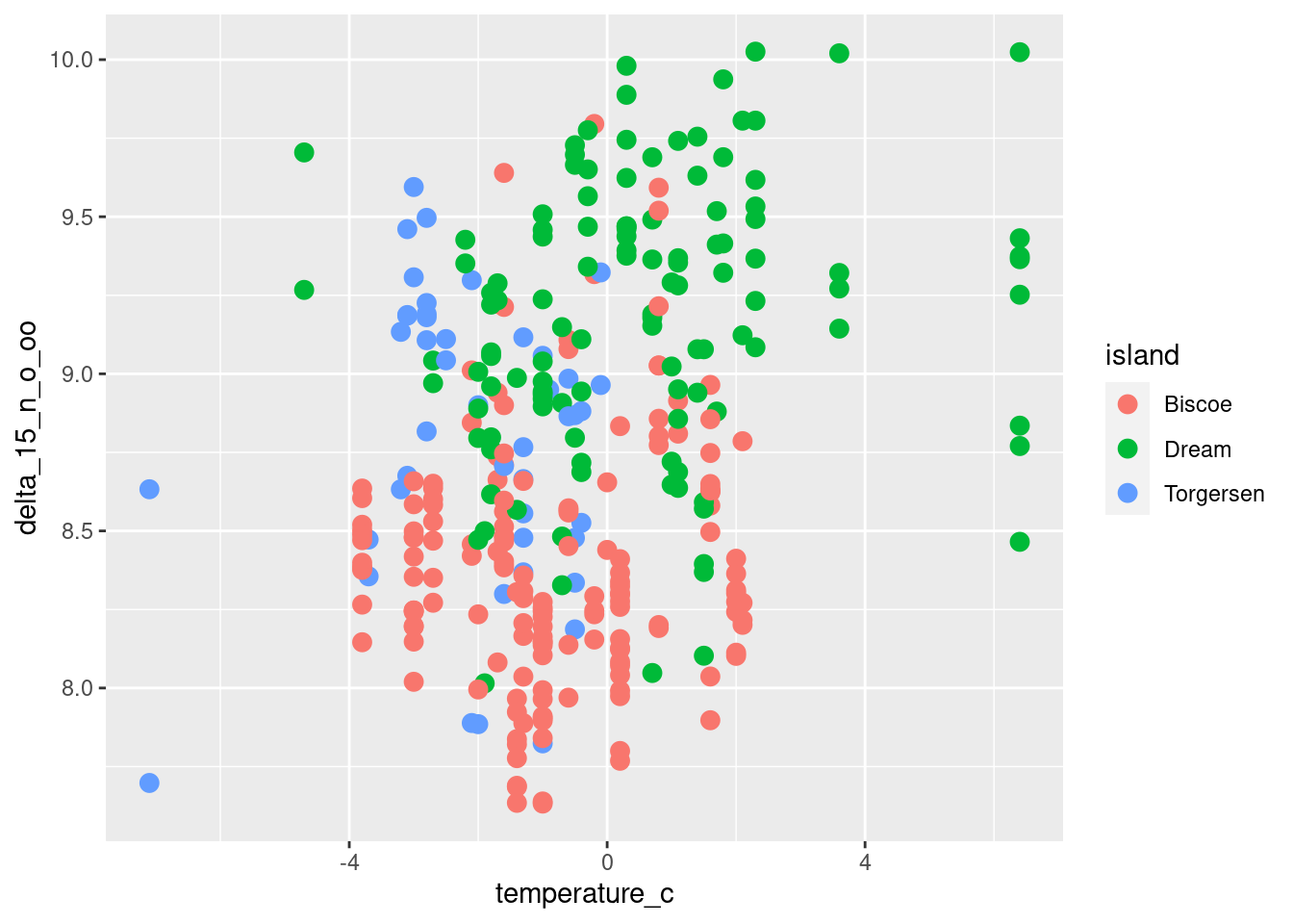
We can finally make our plots. We’re interested in temperatures in comparison to isotope levels. These were in the columns Delta 15 N (o/oo) and Delta 13 C (o/oo) in the original penguins_raw data frame before the column names were cleaned. Which type of plot do you think is most appropriate here? Add some color to show the differences between the 3 islands.
Isotope plots
Make 2 plots. One comparing temperature to Delta 15 N, and one comparing temperature to Delta 13 C. Assign the data from each island to its own color.
# Delta 15 plot
ggplot(penguin_temps,
       aes(x = temperature_c, y = delta_15_n_o_oo, _______ = _______ )) +
  geom_*****(size = 3)

# Delta 13 plot
ggplot(penguin_temps,
       aes(x = temperature_c, y = ......
# Delta 15 plot
ggplot(penguin_temps,
       aes(x = temperature_c, y = delta_15_n_o_oo, color = island)) +
  geom_point(size = 3)


# Delta 13 plot
ggplot(penguin_temps,
       aes(x = temperature_c, y = delta_13_c_o_oo, color = island)) +
  geom_point(size = 3) +
  scale_color_discrete(type = c("green", "blue", "purple"))
Expedition complete
Congratulations! You have learned a bit about how temperature may affect penguin chemistry.
Time to prep for the next expedition…